Farm Water Usage in Honeycomb

Nov 01, 2023

Exploring Aggregate Water Usage Across Australian Farms using Honeycomb

Farm Datasets

In my deep dive into Australian water usage, I stumbled upon a comprehensive dataset from the Department of Agriculture, Fisheries and Forestry in the Australia Government capturing an extensive range of farms across the continent.¹ It is a national compilation of catchment scale land use data for Australia (CLUM), as at December 2020.

Using kepler.gl, we can visualise all the farms in the dataset. Here I am only visualising the Australian State of Victoria, since visualising the entire continent is rather computationally demanding.

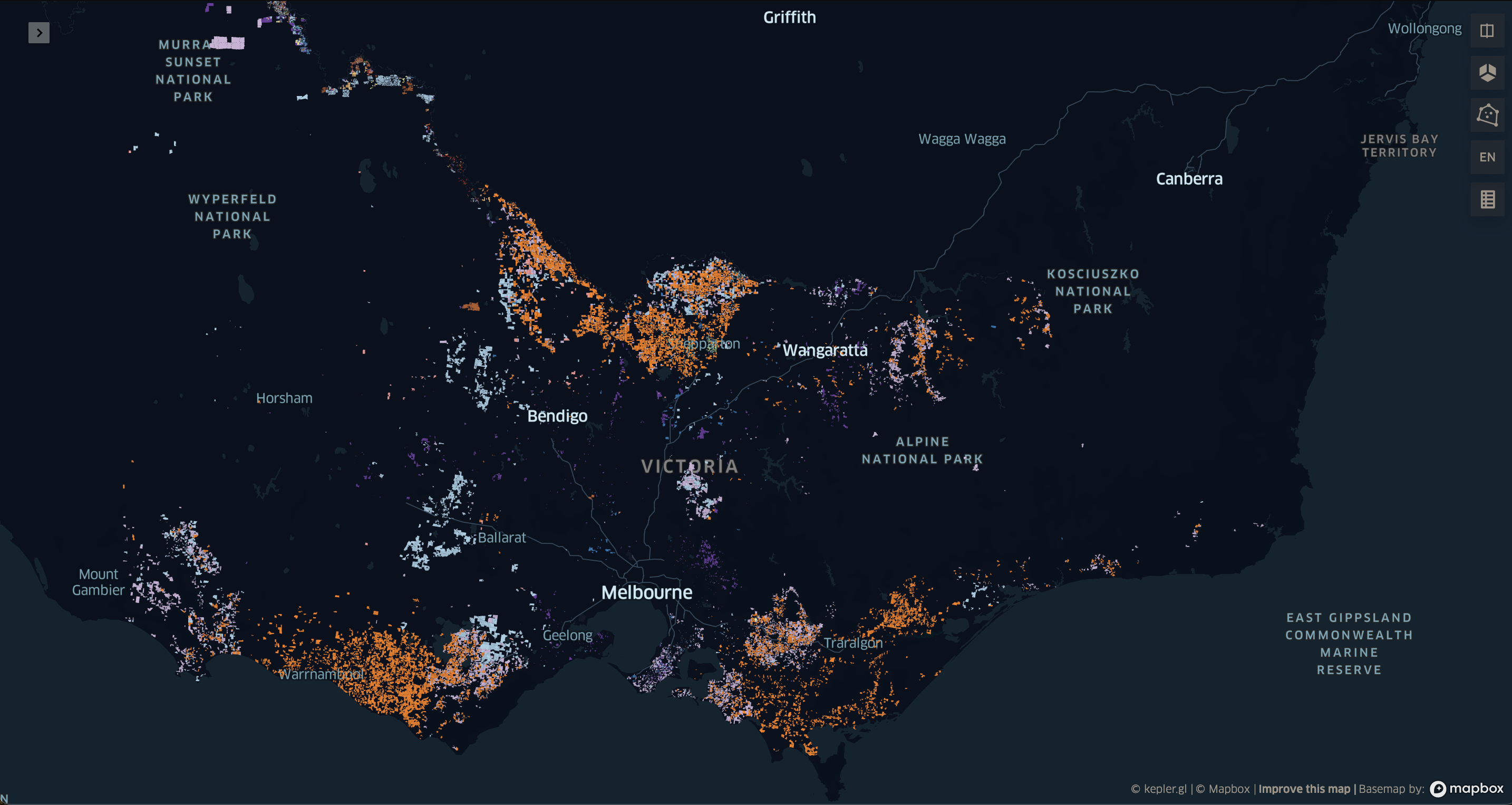
The CLUM dataset is rich with information, containing each farm on the Australian continent represented by a distinct polygon, encompassing a diverse range of agricultural operations. These include various types of crops as well as a variety of livestock, such as cattle, pigs, and chickens.

Each crop and raised animal requires different quantities of water, and this can vary over the course of a growing season. In addition, water usage changes based on the temperture, with cattle and sheep requiring up to 80% more water in extreme temperatures.²

Water Usage

In my next research phase, I focused on sourcing a dataset that detailed the water requirements for different crops, measured in megalitres (ML) per hectare, acre, or square meter. Unfortunately, locating such data from freely accessible sources proved to be a challenging task. Comprehensive datasets encompassing all crop types were notably absent. Consequently, I resorted to searching for each crop individually, delving into various academic studies and agricultural advisories.

For livestock, I had to determine the Stocking Rate per livestock type. This is defined as the number of animals grazing on a given amount of land for a specified time³. I combined this figure with the recommended quantities of water to provide each type of livestock in litres per day². It’s important to note that this approach involves significant assumptions and approximations. There may well be more accurate methods available for estimating this statistic.

Data Transformation Process

Having acquired the raw datasets, my next step involves transforming them into a singular, cohesive dataset.

To begin, I import these datasets into a Jupyter notebook. The CLUM dataset is a shape file (.shp) and will require the python package geopandas to read. The water_usage dataset is a simple csv file and can be easily read using standard pandas.

import geopandas as gpd
import pandas as pd
farm = gpd.read_file("../raw/CLUM_Commodities_2020/CLUM_Commodities_2020.shp")
water_usage = pd.read_csv("../input/water_usage.csv")

Next, I execute a left join operation, merging the water_usage dataframe with the farms dataframe. This is done by using the crop field as the key for the join, ensuring that each record in the farms dataframe is matched with corresponding water usage data based on the type of crop.

farm = farm.merge(water_usage, on='crop', how='left')

We now have a comprehensive dataset that includes each farm, along with the corresponding water usage data for each type of crop.

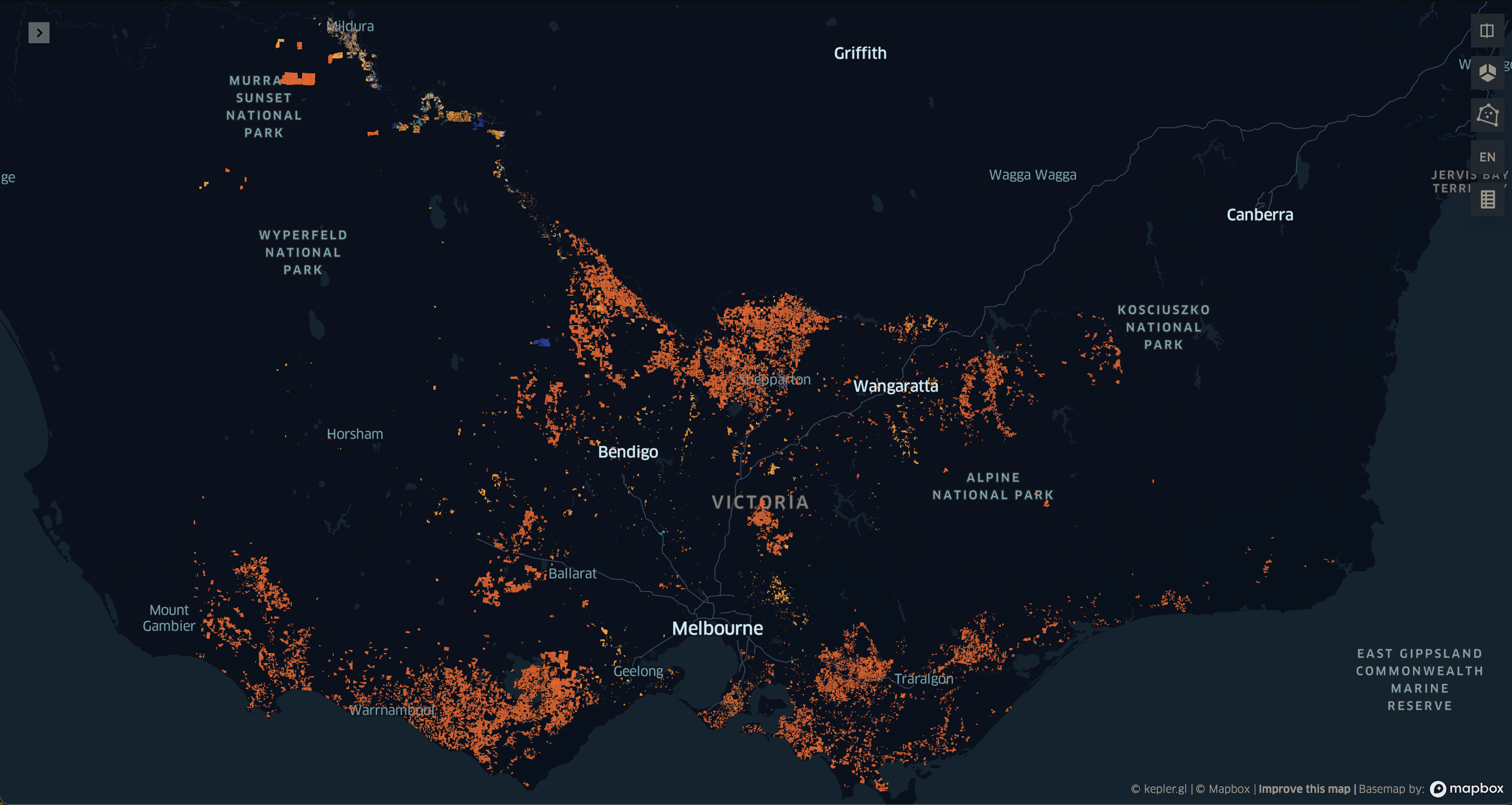
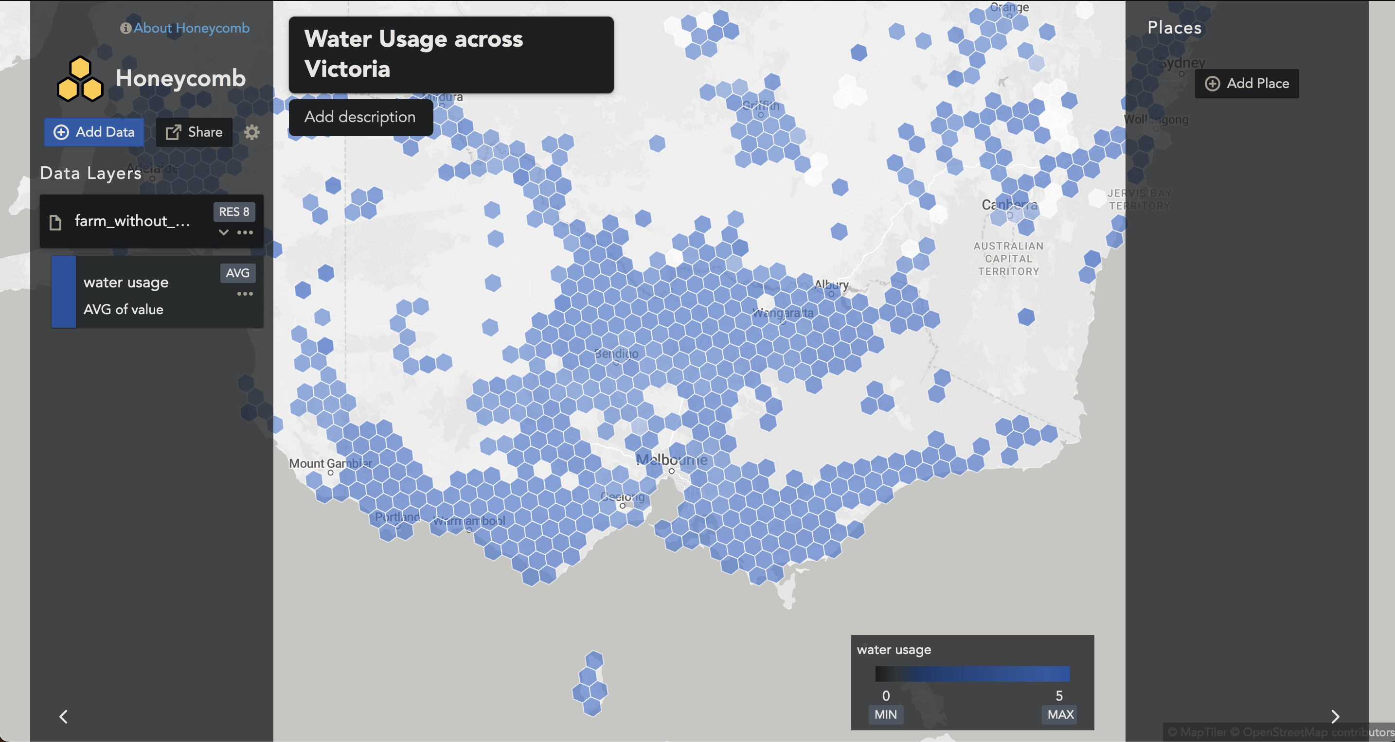
Interpreting this map presents a challenge. It depicts a patchwork of colours, where we can see some farms utilise significantly more water than other, and, with some difficulty, see which areas in the State where more water is used.

What I want to see is water usage reduced to a standardised unit, like a square, in which I can clearly see regions with higher water usage, without the distraction of the farm polygons.

Honeycomb

To visualise my final dataset, I employed Honeycomb, an advanced mapping analytics tool developed by Carston Hernke of Maps and Data LLC. Honeycomb stands out as a complimentary mapping platform leveraging the H3 hierarchical geospatial indexing system, a framework initially developed by Uber. This innovative tool excels in presenting geospatial datasets, specifically those aggregated to the H3 hexagonal unit. It enables the importation of various data layers into its platform, facilitating the creation of synthetic layers that are a combination of your datasets. This synthetic layer is an effective tool to compare and contrast statistics across an extensive region.

Here is an embedded Honeycomb map, depicting population statistics in San Francisco.

To give a concrete example, consider someone working in the Real Estate industry who aims to analyse the relationship between average home sale prices and average rental rates in a specific region. This analysis could help determine if the home prices in a particular area are proportional to the rental rates. To do this, one would obtain data on sale prices and geospatial coordinates (longitude and latitude) of each property sold. Similarly, you would gather the rental price, noting the coordinates of rented properties.

The next step involves aggregating this data within a defined geographic area, such as a hexagon, and calculating the average home sale price within that area. By comparing this figure with the average rental price in the same hexagon, it’s possible to identify significant disparities between the two across a large region with many thousands of properties and rental contracts. This methodology underscores the importance of obtaining highly detailed, granular data. The finer the granularity of the data, the more precise and accurate your analysis will be, ensuring the retention of fidelity in your measurements.

Hexagons

But first, we need to add the corresponding H3 hexagons to the dataset. To do this we employ the H3 python package, and use a function called polyfill. This determines which hexagons fit entirely wihin the bounds of each farm polygon, and left join the corresponding h3 index. The explode parameter confirms we are happy with this rather expansive left join.

import h3
farm = farm.h3.polyfill(8, explode=True)

Now we are ready to visualise the dataset with Honeycomb.

Visusalisation

Creating a map with Honeycomb is super simple.

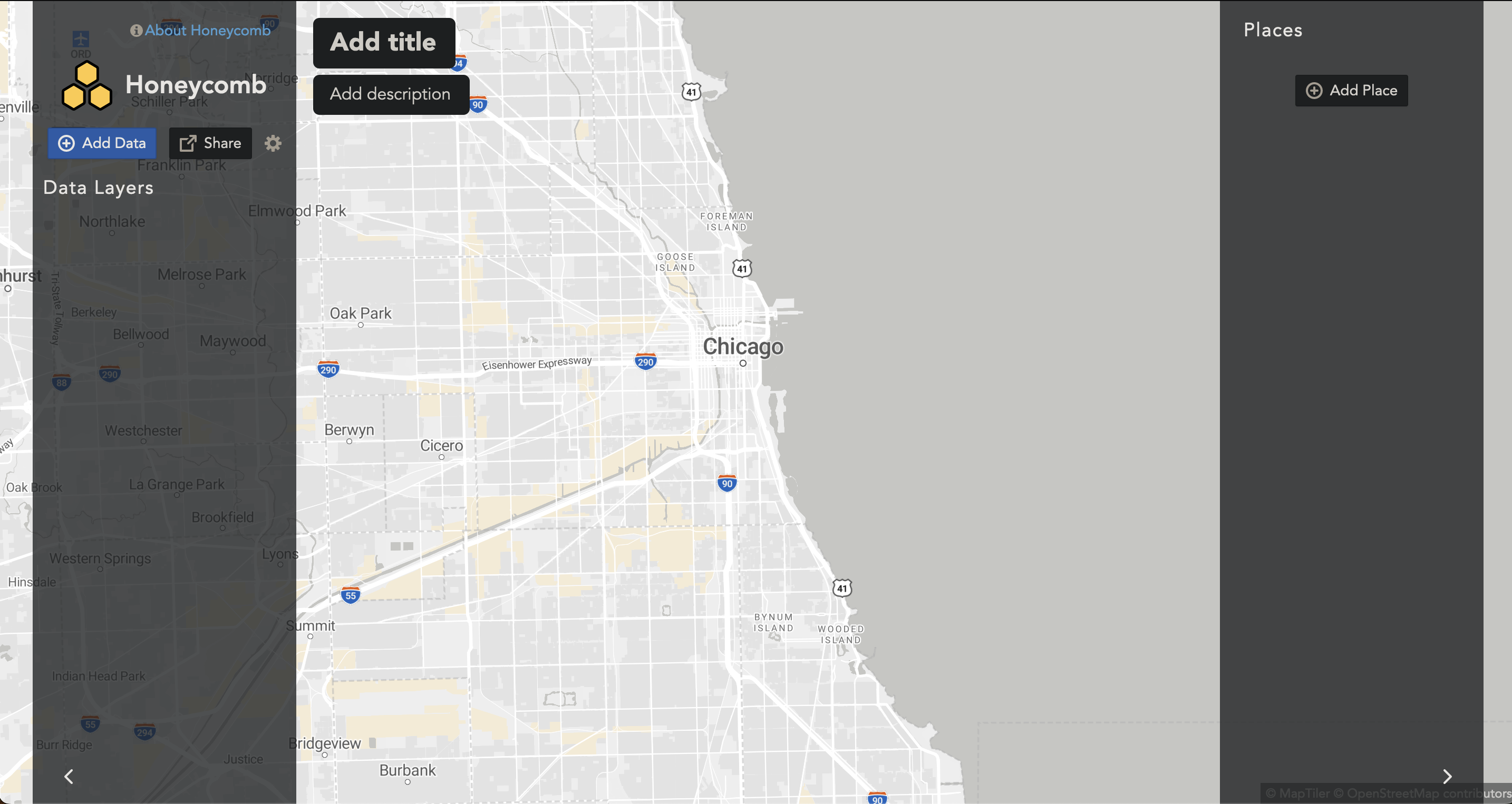
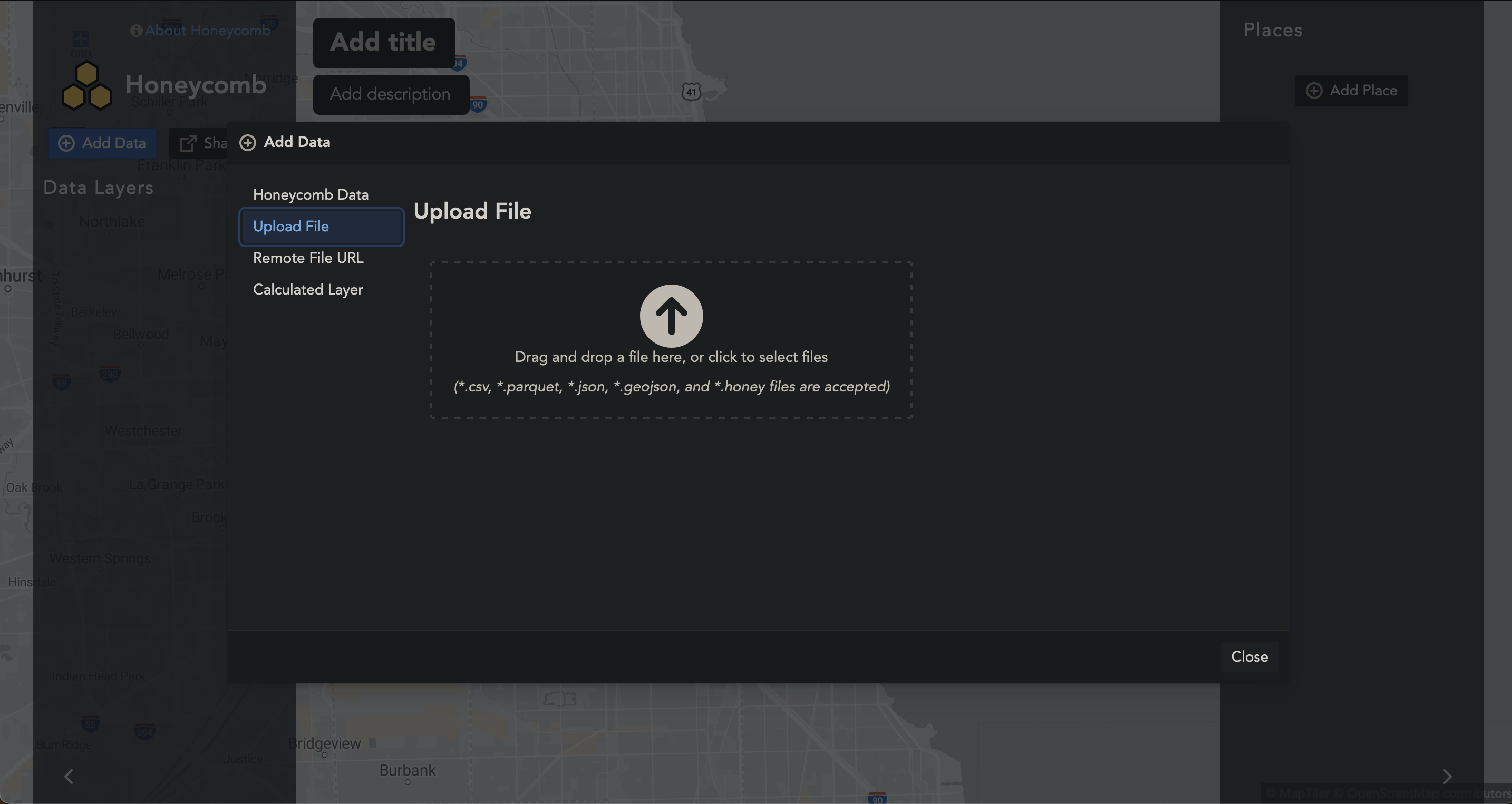
First we upload our farms.csv into the browser. Honeycomb supports many types of raw datasets, including .csv, .parquet, .json, and .geojson. One great thing about Honeycomb is that your data is safe, since your data never leaves the browser.

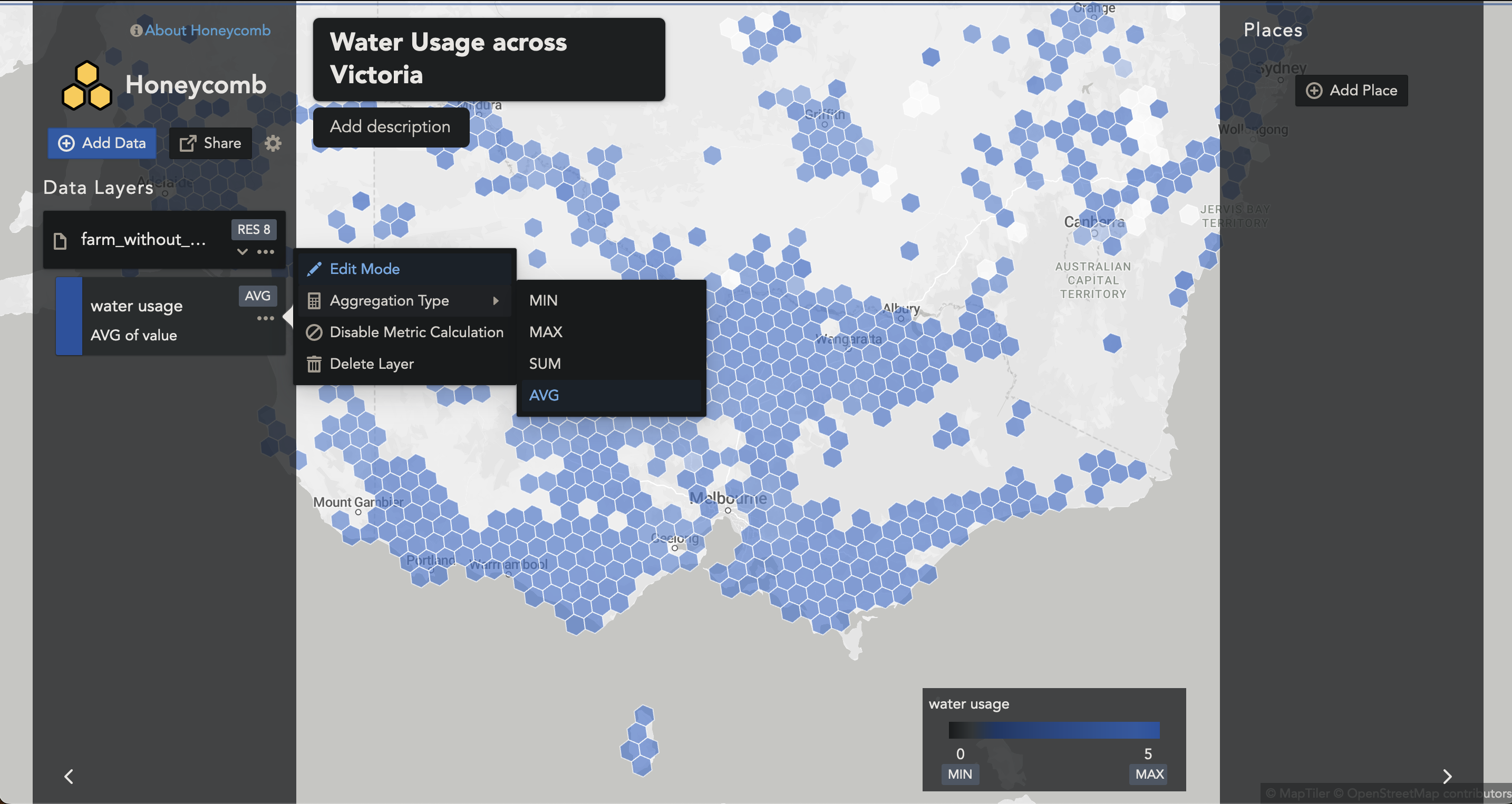
Once uploaded, our water_usage column is automatically formatted to AVG. This means as one zooms in and out, the hexagons in that corresponding area will be averaged. This is not what we want.

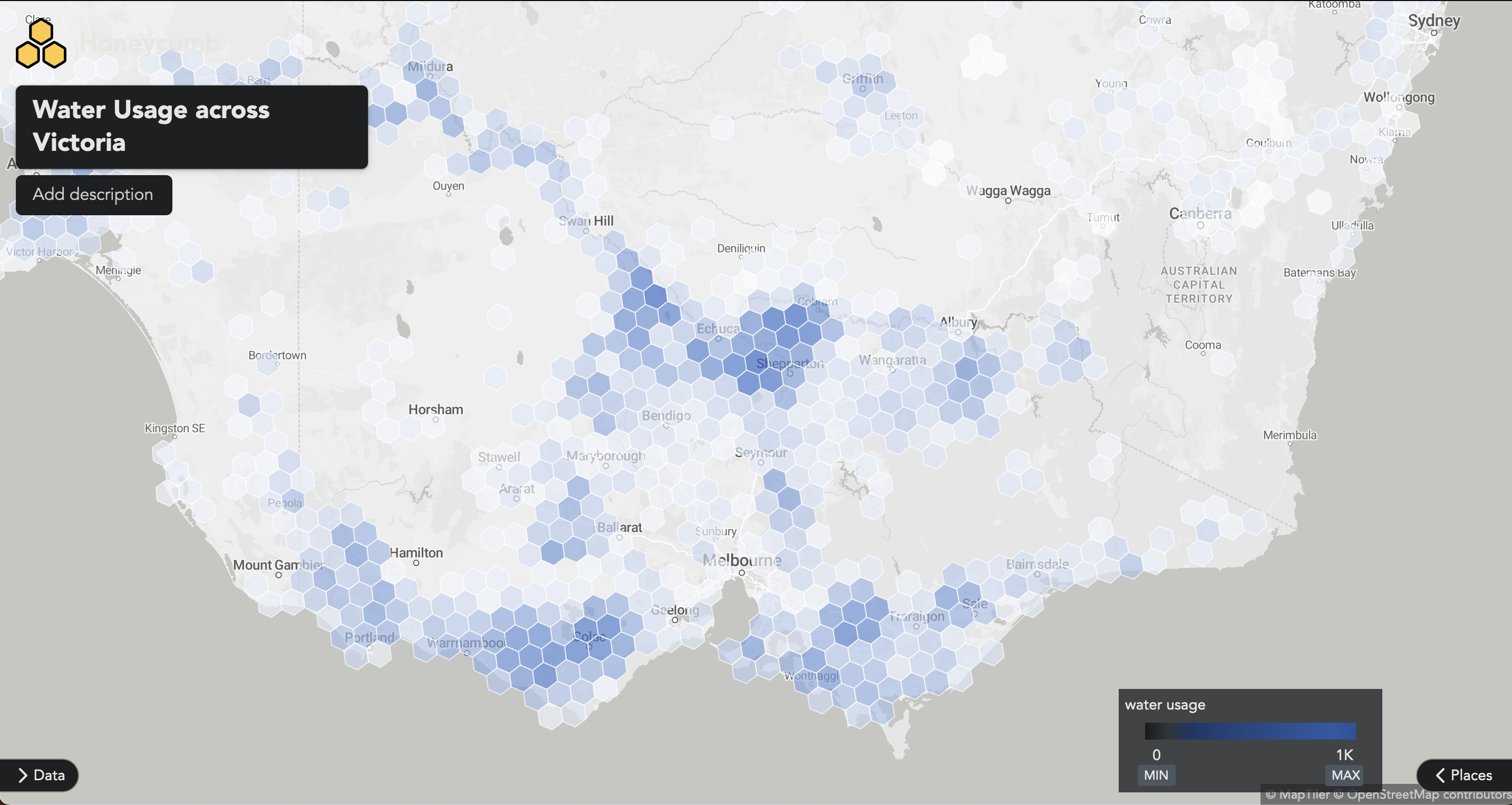
To change to a SUM, we can select the Aggregation Type to SUM.

Now we can zoom in and out and see the hexagons adding together. The colour automatically scales to the range of values you provide in your dataset. In this case the range is in megalitres (ML). While we’re at it, we can toggle away the Data and Places, and see the map in all its glory.

Zooming into a region in Victoria, just above Bendigo, we can further explore the water usage in the region.

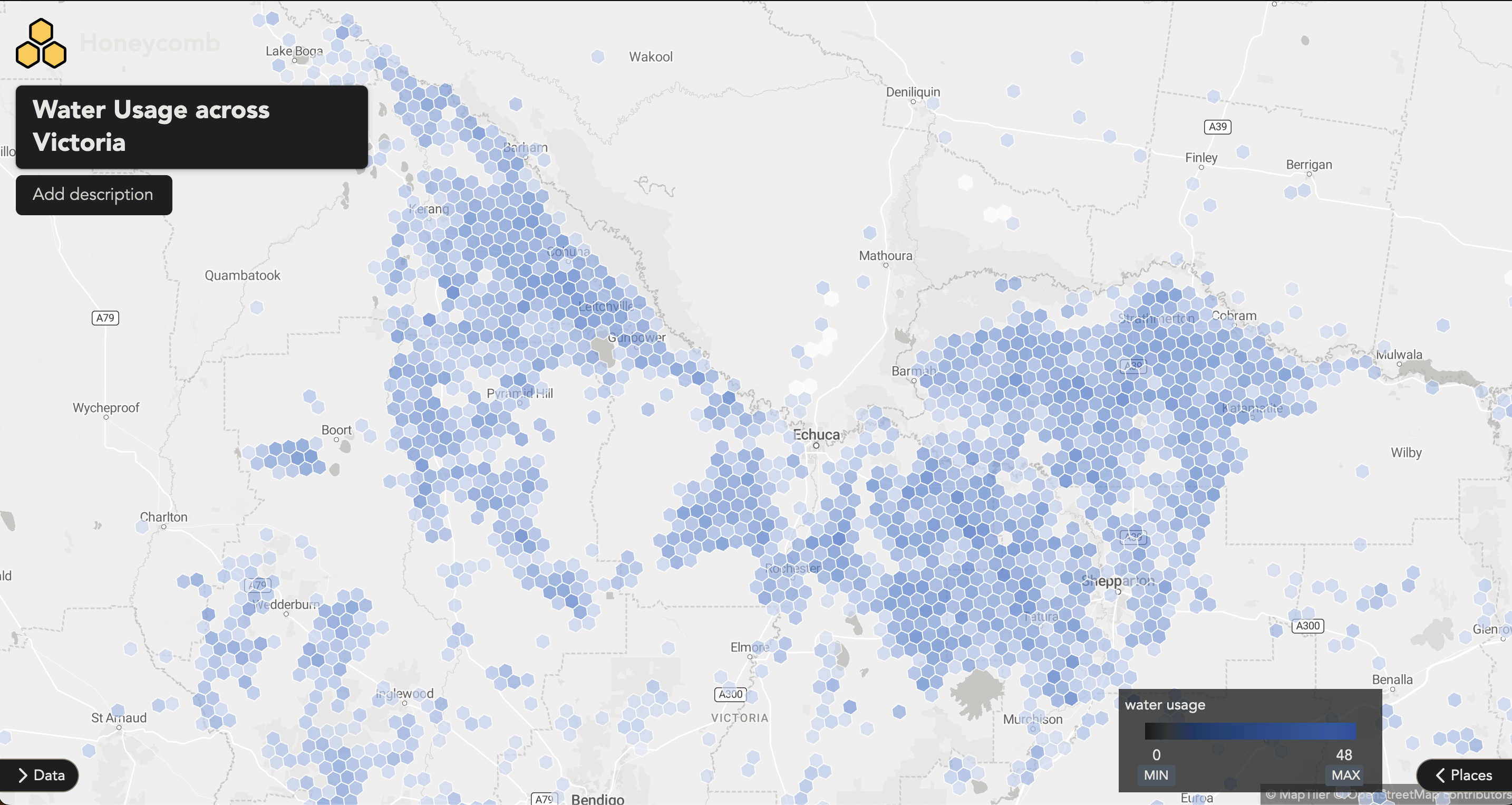
This approach provides us with a powerful tool to evaluate farm water usage across the entire expanse of Australia.

I welcome any feedback or inquiries about this project. Feel free to contact me at hello@alexryan.com.au.

References